For the last couple years, I’ve used the audio editor Audacity to provide myself with some very detailed examinations of the notes and timing of the Great Highland Bagpipe.

I’ve used the approach to figure out which embellishments were being played in unpublished scores, determine/confirm where the beat was being placed in the flow of notes, check out the internal timings of embellishments,  and, most recently, I’ve looked at pulsing.  I’ve refined the mechanics of working with Audacity and will share it here.

To go down this path yourself, you’ll need two things:

1. A copy of Audacity running on a computer. It’s free and runs on Windows, Mac and Linux.
2. A digital music file source in a file that Audacity can import. Your options are almost limitless here. A clean solo bagpipe recording is the best starting point. (Note: I use MP3s which I might “rip” from my large CD/LP collection or from YouTube. When needed, I use a low cost set of flexible and capable tools by Applian Technologies.)

Get Audacity set up and running. Then open your digital music file in Audacity.  Once the file is open, do the following operations using the tool bar across the top window:

1. Select, Tracks, All.
2. Tracks, Mix, Mix down to Mono.
3. Effect, Normalize, Normalize Peak Amplitude to 0.0, Apply.
4. Move cursor to left of waveform (Track Control Panel) and right click. Select Spectrogram.
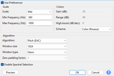
5. Move cursor to left of waveform (Track Control Panel) and right click. Select Spectrogram Settings as shown in attached screen shot.  (You can save these as a preset.)

When you click on OK, you should see something like the screenshot below. This is a march peformed by a well known player at a prestigious event. We’re not going to look at details here, but will just getting an idea of the layout.

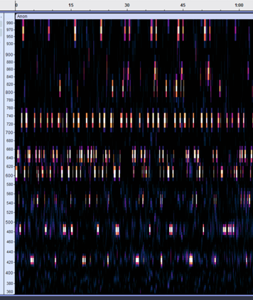
On the left (vertical) axis are the number of cycles per second (i.e., Hz) as related to the pitch of the note.  The low notes are at the bottom of the chart and the high notes along the top. As there are nine notes, we see nine horizontal stripes of bright dots.  The highest row is HighA at about 970 Hz. The lowest row is LowG at about 425 Hz. The second one up is LowA at about 485 Hz. The remaining notes (approximate Hz) are B ( 545), C (607), D (650), E (730), F (810), and HighG (850). This tune accesses every note in the scale. The horizontal axis is time. If you look closely, you’ll see that the notes are played in one after the other to make a melody. This piece of music takes about a minute to play.

Now we’ll look with more detail into the durations of the notes.  The figure below shows the second line of Scotland the Brave as played by another prominent piper. It’s greatly magnified compared to the graph above.  Below the graph, I’ve posted the musical notation being played. Remember that the graph is linear in time, while staff notation is not, so the notes don’t line up particularly well from one to the other. 

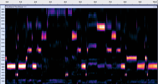
There is a taorluath at about 0.7 seconds between two LowAs.  You can clearly see the LowG, D, LowG and E.  There’s a Low A followed by a C doubling just after 2.0 seconds – note the short HighG (gracenote) to a brief C followed by a very short D (gracenote) and the rest of the C melody note.  There’s a grip (leumluath) at 4.0 seconds between two HighAs – and so forth.

Hopefully, this quick overview will give you an appreciation for how this technology might be used to answer some interesting questions.  One could imagine that, if automated, this sort of close examination could be used for teaching and/or technical assessment.

You may also know that there are several flavors of digital bagpipes available today that don’t need the analog to digital conversion we’ve done here. Matt Willis, Bagpiper put together a comparable evaluation of Scotland the Brave using a midi bagpipe and controller. It’s really interesting to see how closely the approach above compares.

Steve MacLeod, copyright 2025